Neural Network Basics and Multi-Layer Perceptron

Artificial Neurons

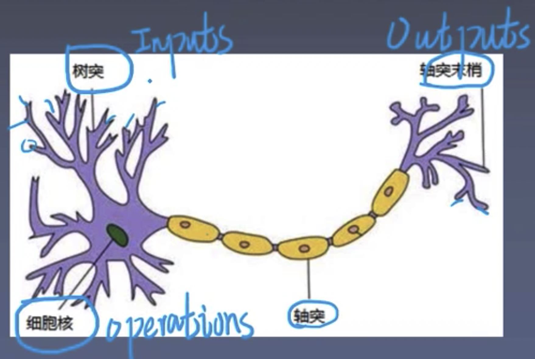
Artificial Neuron: A mathematical model abstracted from human neurons.

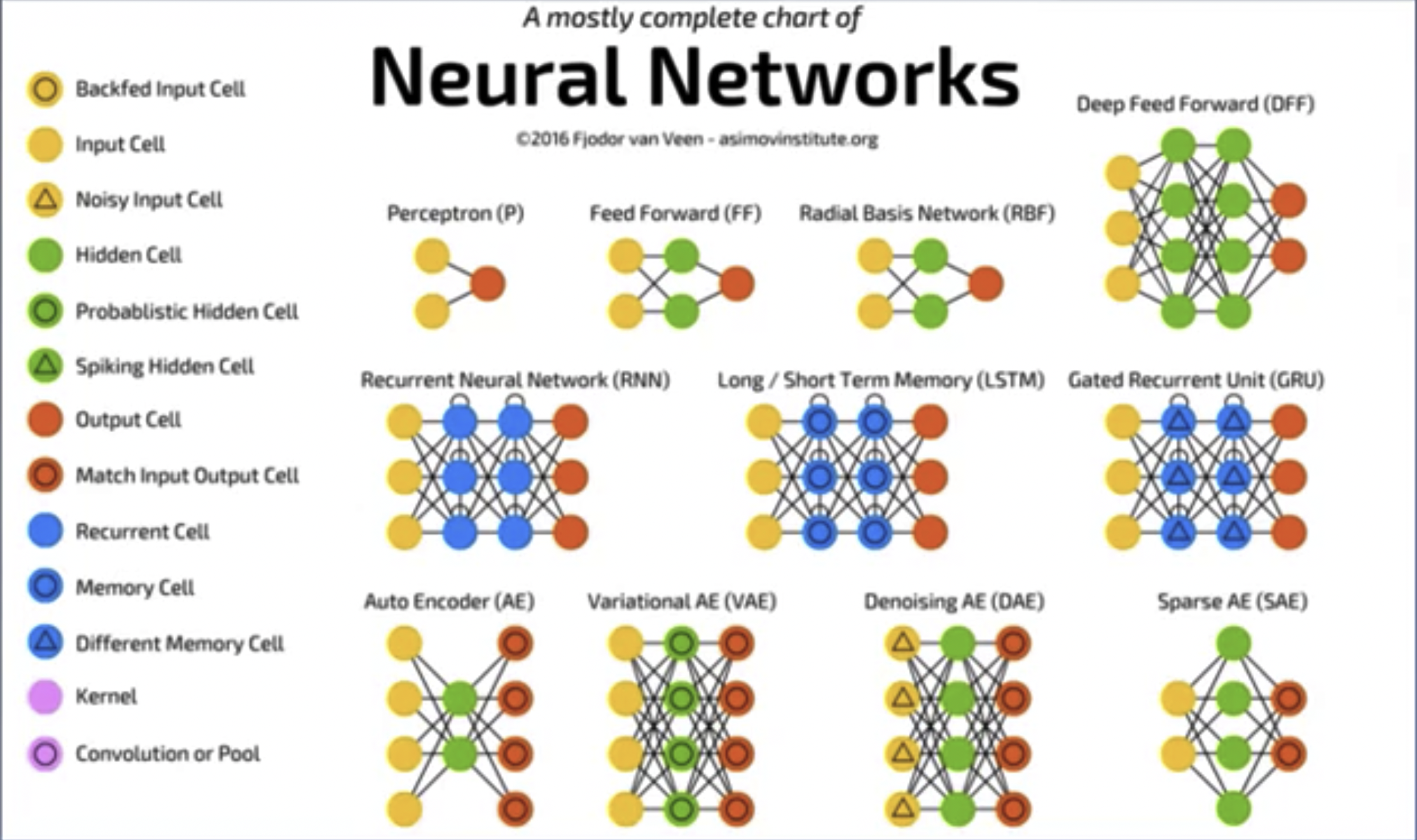
Artificial Neural Network: A machine learning model composed of a large number of neurons connected in a certain way.

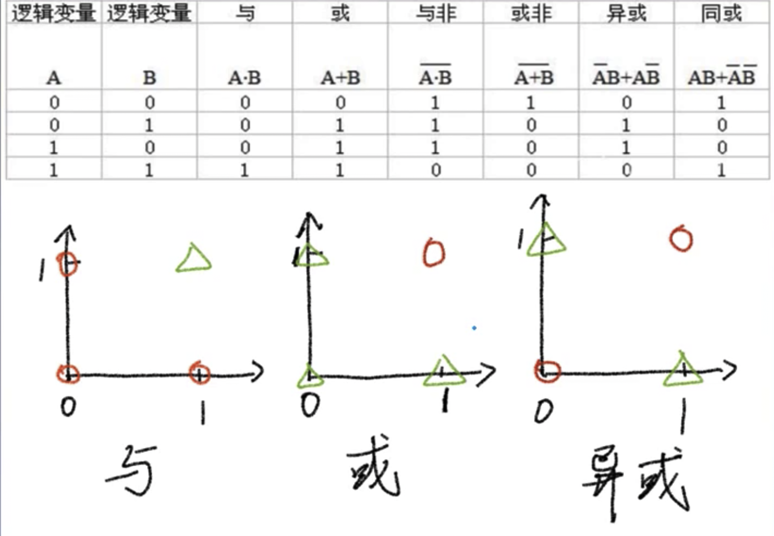
Minsky proved in 1963 that Perceptron cannot solve the XOR problem.

Multi-Layer Perceptron

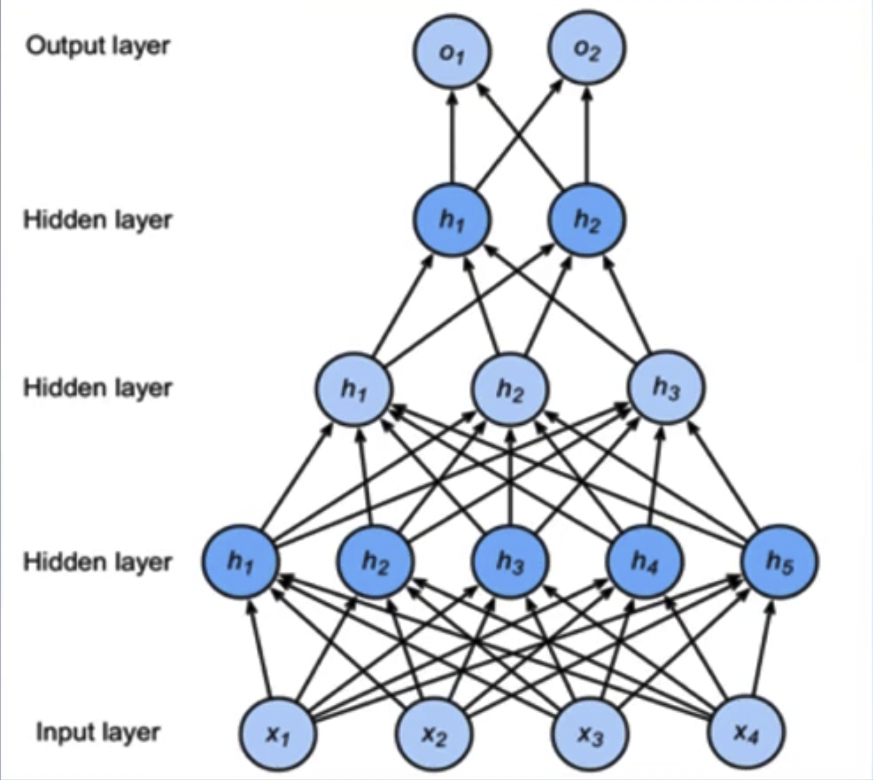
Multi-Layer Perceptron (MLP): Introduces one or more hidden layers based on a single-layer neural network, resulting in multiple network layers, hence the term multi-layer perceptron.

Forward propagation of MLP:

Activation function of MLP: Without activation function, the network degenerates into a single-layer network:
$$ H = XW_h + b_h $$ $$ O = HW_o + b_o = (XW_h + b_h)W_o + b_o = XW_hW_o + b_hW_o + b_o $$
Adding activation function to hidden layer can prevent network degeneration:
$$ h = \sigma(W_1x + b_1) $$ $$ o = \mathbf{w}_2^T h + b_2 $$

Activation Function

Makes MLP truly multi-layered; otherwise, it’s equivalent to a single layer.

Introduces non-linearity, enabling the network to approximate any non-linear function (universal approximator theorem).

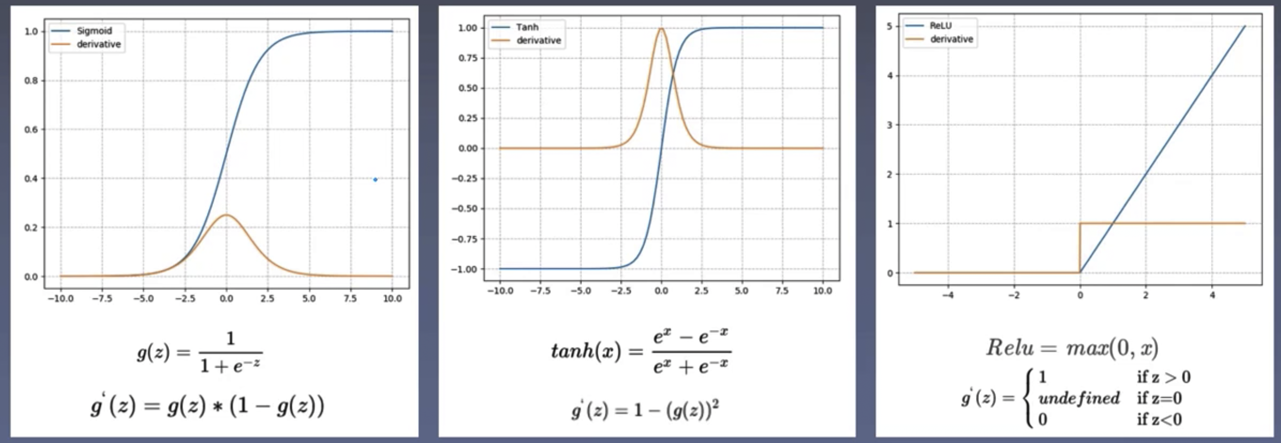
An activation function should have the following properties:

Continuous and differentiable (a few points can be non-differentiable) to facilitate numerical optimization methods for learning network parameters.
The activation function and its derivative should be as simple as possible to enhance computational efficiency.
The range of the derivative of the activation function should be in a suitable range, neither too large nor too small, to ensure training efficiency and stability.

Common activation functions: Sigmoid, Tanh, ReLU (Rectified Linear Unit):

Backpropagation

Forward propagation: Data starts from the input layer and gradually passes to the output.

Backpropagation: Gradients are passed backward from the loss function to the first layer.

Purpose of backpropagation: Used for weight updates to make the network output closer to the labels.

Loss Function

Measures the difference between the model output and the true labels.

$$ Loss = f(\hat{y}, y) $$

Principle of Backpropagation

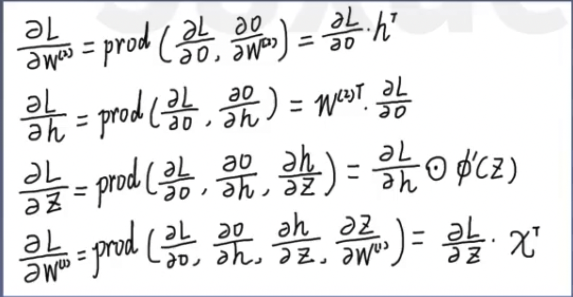
Chain rule in calculus:

$$ y = f(u), u = g(x) $$ $$ \frac{\partial y}{\partial x} = \frac{\partial y}{\partial u} \frac{\partial u}{\partial x} $$

Network computation graph:

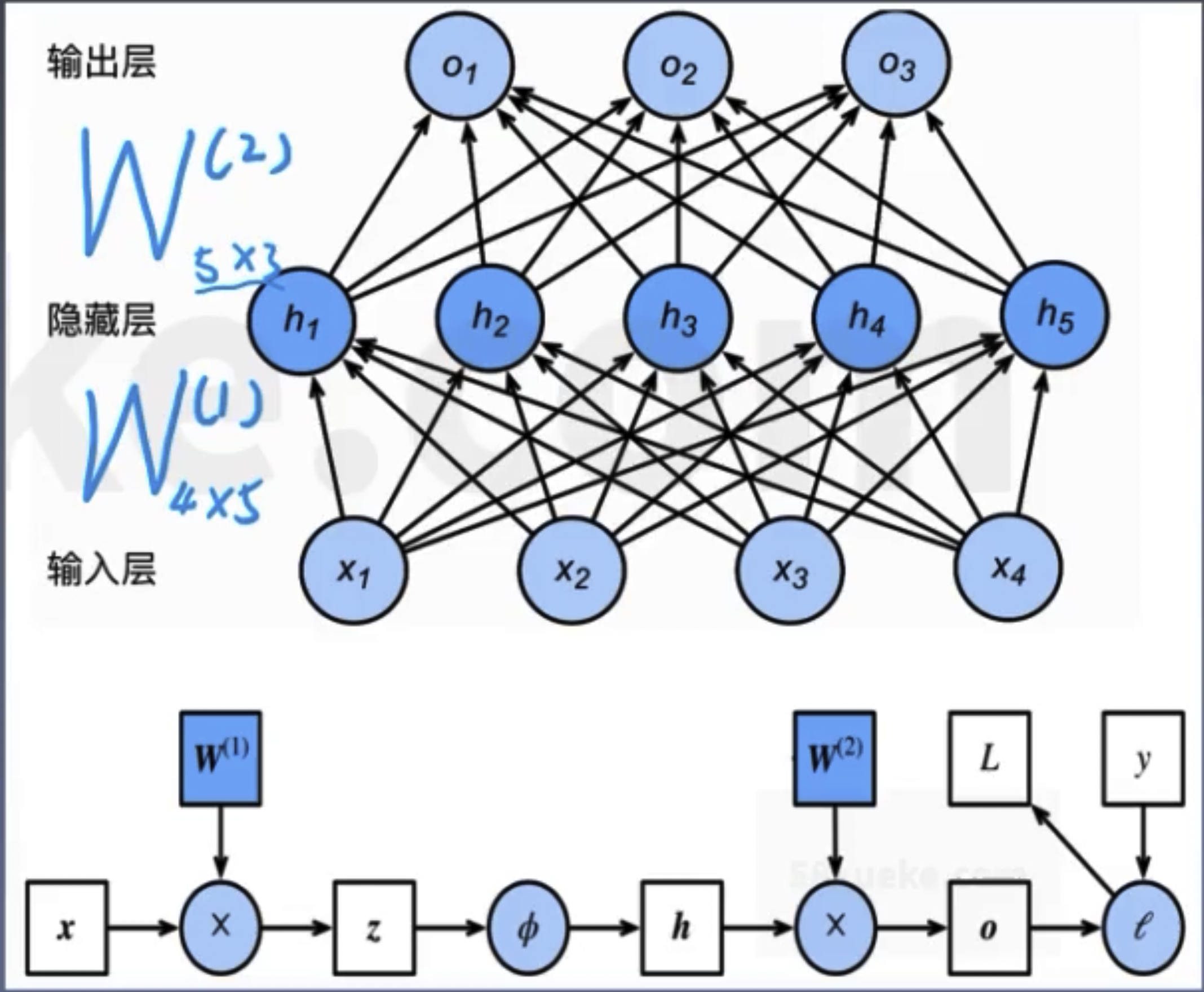
Definition of computation symbol: prod(x,y), represents multiplying x and y after necessary shape transformations.

Gradient Descent

Weights are updated along the negative gradient direction to reduce the function value.

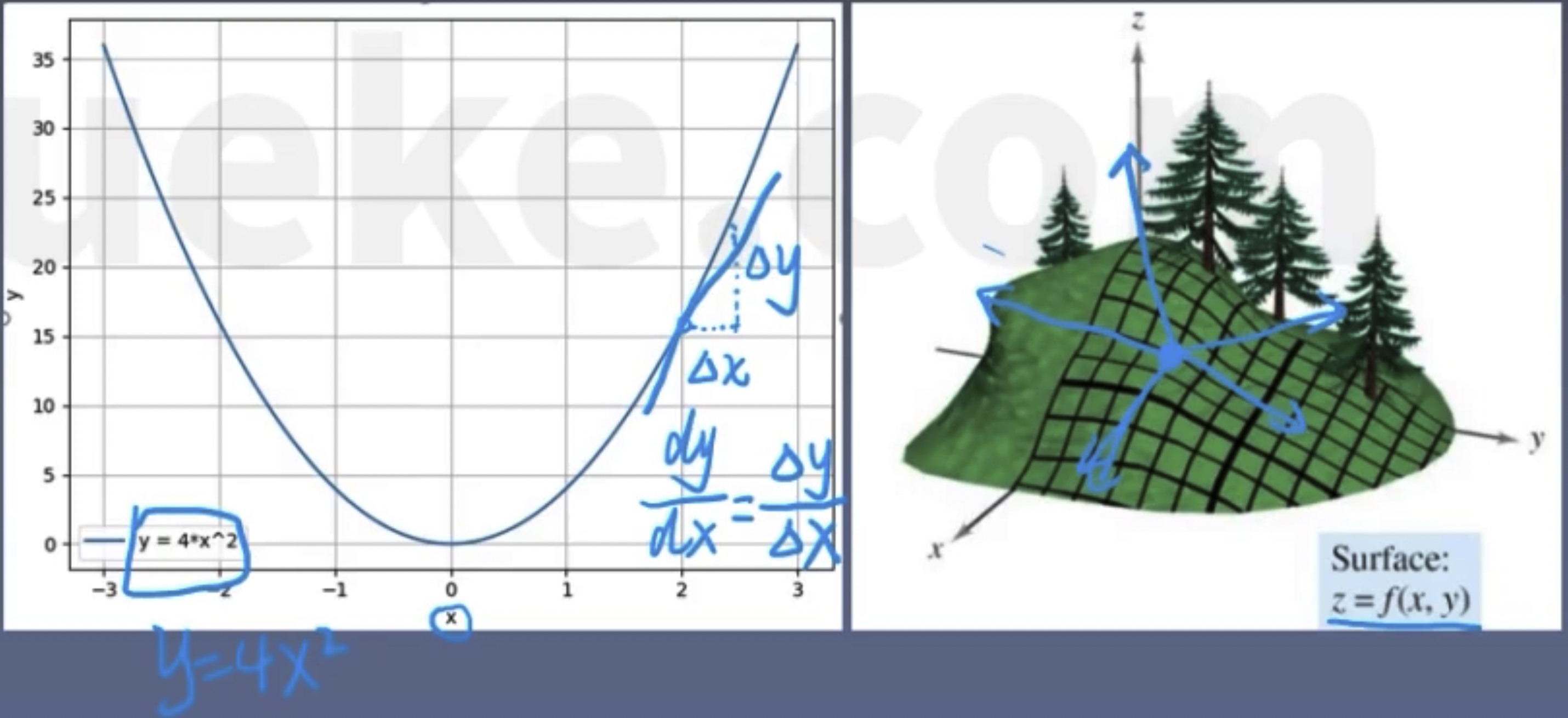
Derivative: The rate of change of a function with respect to a coordinate axis.

Directional derivative: The rate of change in a specified direction.

Gradient: A vector, the direction in which the directional derivative is maximized.

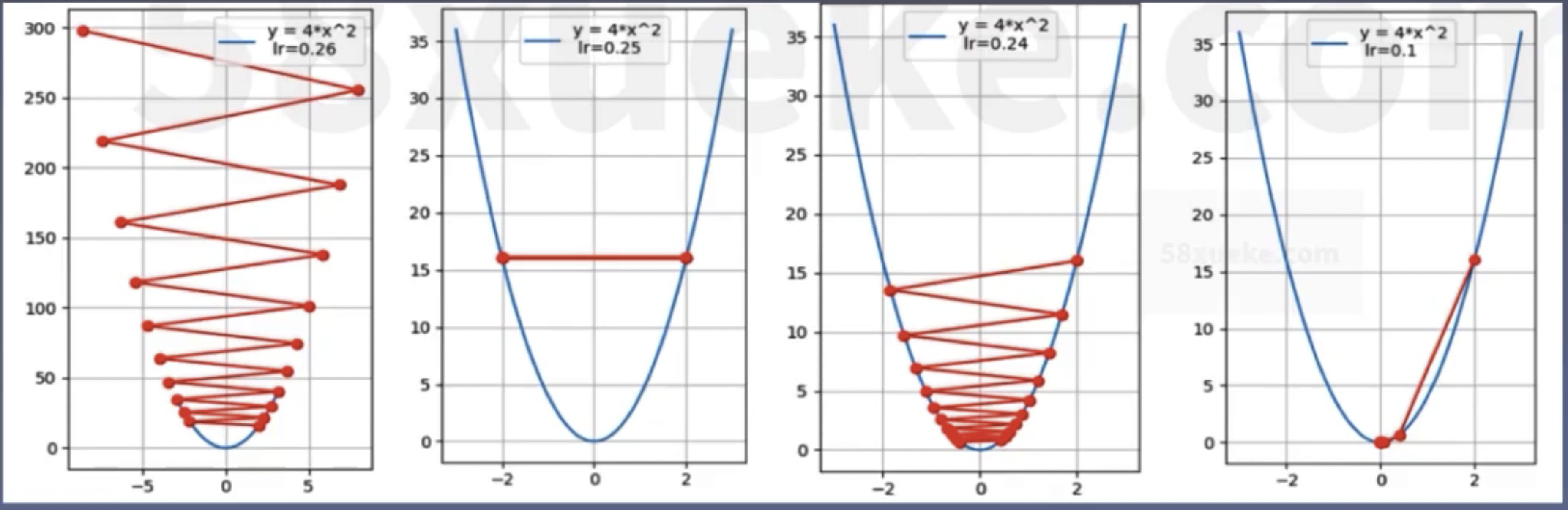
Learning Rate

Learning rate (LR): Controls the step size of the update.

Without learning rate:

$$ \mathbf{w}_{i+1} = \mathbf{w}_i - g(\mathbf{w}_i) $$

With learning rate:

$$ \mathbf{w}_{i+1} = \mathbf{w}_i - \text{LR} \cdot g(\mathbf{w}_i) $$

Loss Function and Objective Function

Measures the gap between model output and true labels.

Loss Function

$$ Loss = f(\hat{y}, y) $$

Single sample.

Cost Function

$$ Cost = \frac{1}{N} \sum_{i=1}^N f(\hat{y_i}, y_i) $$

Overall samples.

Objective Function

$$ Obj = Cost + \text{Regularization Term} $$

Two Common Loss Functions

MSE (Mean Squared Error): The mean of the squared differences between the output and the labels, often used in regression tasks. Formula:

$$ MSE = \frac{1}{n} \sum_{i=1}^n (y_i - \hat{y_i})^2 $$

Example: label = (1, 2) pred = (1.5, 1.5)

$$ MSE = \frac{(1 - 1.5)^2 + (2 - 1.5)^2}{2} = 0.25 $$

CE (Cross Entropy): Derived from information theory, used to measure the difference between two distributions, often used in classification tasks. Formula:

$$ H(p, q) = - \sum_{i=1}^n p(x_i) \log q(x_i) $$

Cross entropy’s good partner – Softmax function: Converts data to a form that conforms to a probability distribution.

Properties of probability:

Probability values are non-negative.
The sum of probabilities is 1.

Softmax Function

Converts data to a form that conforms to a probability distribution:

Takes the exponent to achieve non-negativity.
Divides by the sum of exponents to achieve a sum of 1:

$$ y_i = S(z)_i = \frac{e^{z_i}}{\sum_{j=1}^{C} e^{z_j}}, \quad i = 1, \ldots, C $$

Weight Initialization

Assigning values to weight parameters before training; good weight initialization is beneficial for model training.

Random initialization method: Randomly initializing weights from a Gaussian distribution, e.g., N~(0, 0.01). The 30-rule: The probability that the value is within (u-3o, u+3o) is 99.73%.

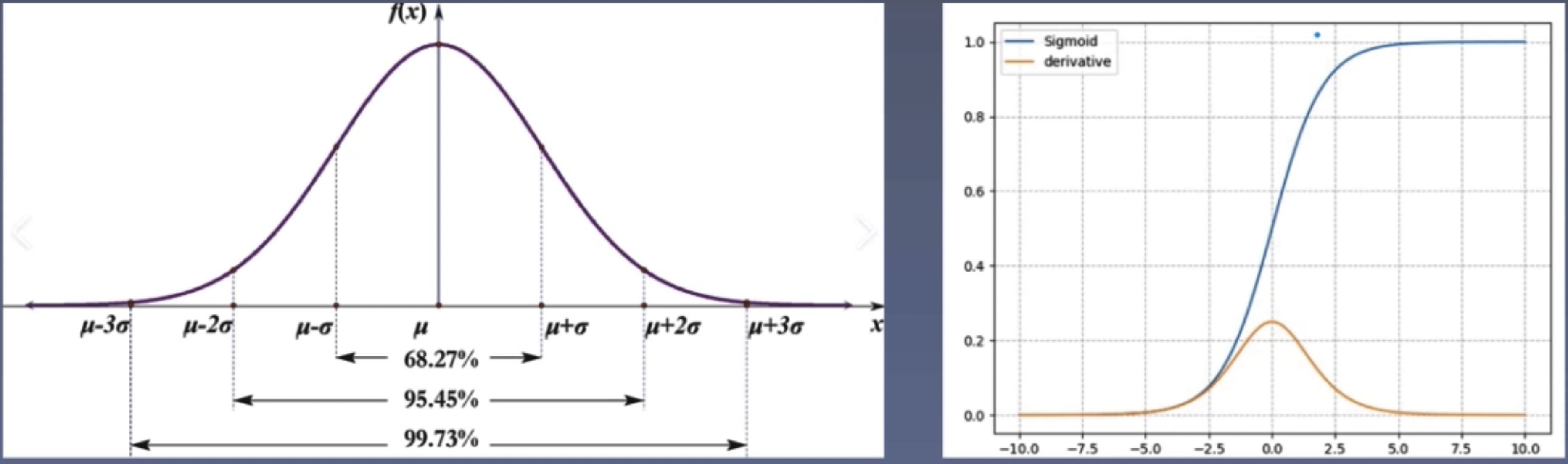
Controlling the scale of weights (key parameter is the standard deviation in the probability distribution) is important because excessively large weights can cause the values to fall into some saturated regions of the activation function, leading to gradient vanishing.

Adaptive standard deviation: The standard deviation in the adaptive random distribution.

Xavier Initialization: From “Understanding the difficulty of training deep feedforward neural networks”:
$$ U \left( -\sqrt{\frac{6}{a+b}}, \sqrt{\frac{6}{a+b}} \right) $$
where a is the number of input neurons, and b is the number of output neurons.
Kaiming Initialization: From “Delving Deep into Rectifiers: Surpassing Human-Level Performance on ImageNet Classification”:

Regularization Methods

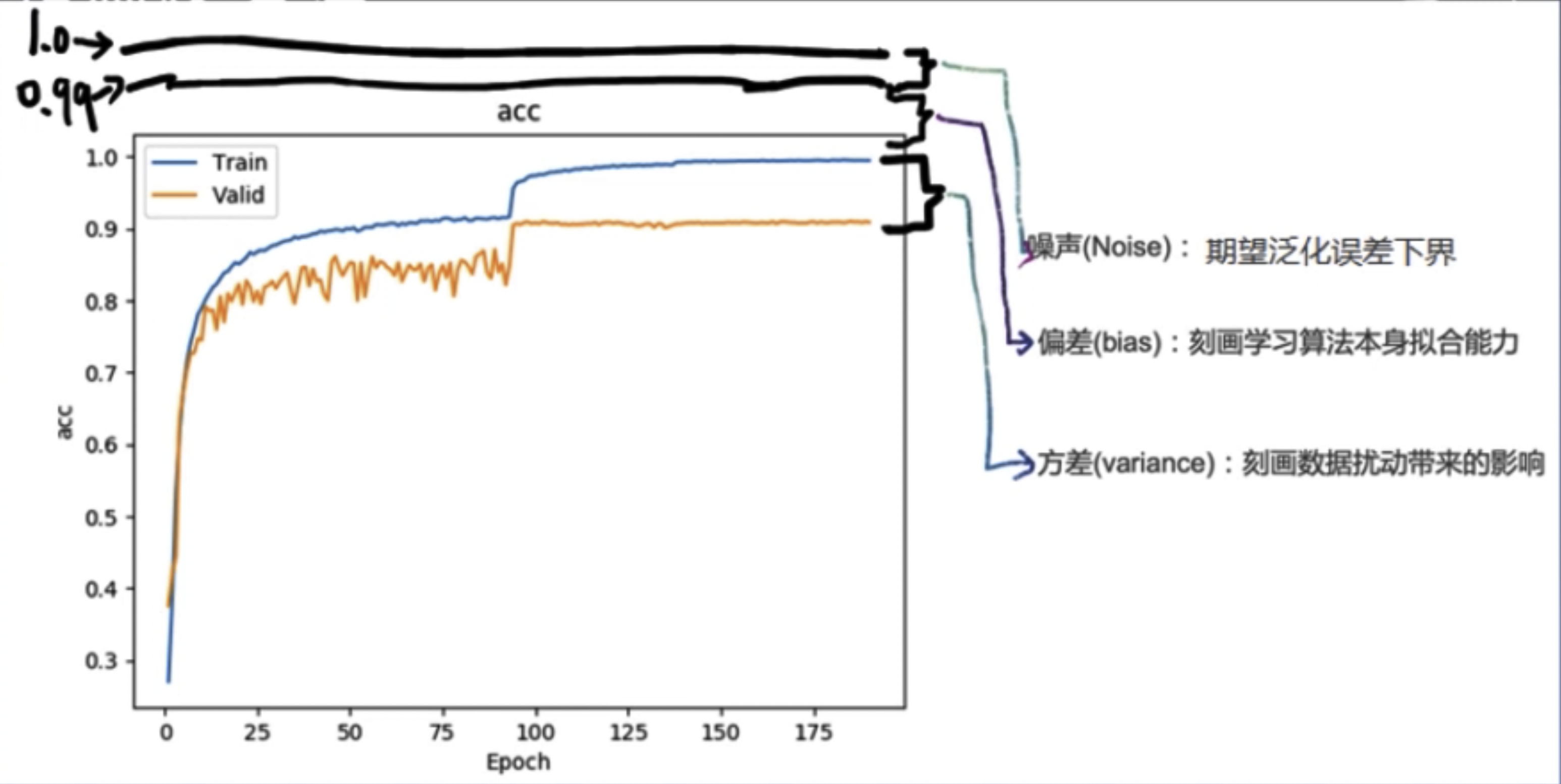
Regularization: Strategies to reduce variance, commonly understood as ways to mitigate overfitting.

Error can be decomposed into: bias, variance, and noise sum. That is, error = bias + variance + noise sum.

Bias measures the deviation of the expected prediction of the learning algorithm from the true result, indicating the fitting ability of the learning algorithm itself.

Variance measures the changes in learning performance caused by variations in the training set of the same size, indicating the impact of data perturbations.

Noise expresses the lower bound of the expected generalization error that any learning algorithm can achieve on the current task.

Overfitting phenomenon: Excessively high variance performs well on the training set but poorly on the test set.

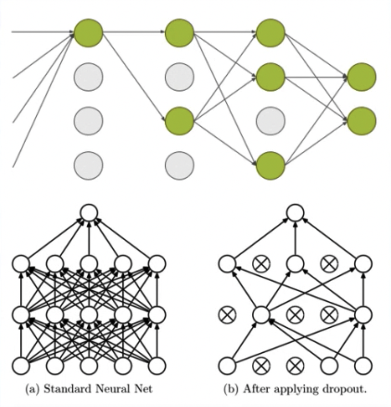
Dropout: Random deactivation

Advantages: Avoids over-reliance on a particular neuron, thereby reducing overfitting.

Random: dropout probability (e.g., p=0.5)

Deactivation: weight = 0

Considerations: Scale changes during training and testing phases. During testing, neuron output values need to be multiplied by p.

Other Regularization Methods:

Batch normalization: “Batch Normalization: Accelerating Deep Network Training by Reducing Internal Covariate Shift”
Layer Normalization: “Layer Normalization”
Instance Normalization: “Instance Normalization: The Missing Ingredient for Fast Stylization”
Group Normalization: “Group Normalization”